But if you need others reading the spreadsheet to be able to see all of the data, then you may be looking for a way to accomplish that quickly. Our tutorial below will show you how to apply the “Wrap Text” formatting to a cell so that Excel will force text onto a new line so that you can see all of it.
How to Force Text to Multiple Lines in Excel 2013
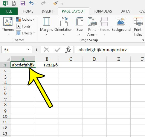
The steps in this article were performed in Microsoft Excel 2013. By completing the steps in this guide you will be selecting a cell or group of cells and applying the “Wrap Text” formatting to it. This will causes the cells to change in size to accommodate any text that is not visible because it is too large for the current cell size. Step 1: Open your spreadsheet in Excel 2013. Step 2: Select the cell or cells containing the text that you would like to wrap.
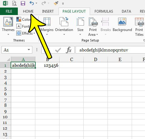
Step 3: Click the Home tab at the top of the window.
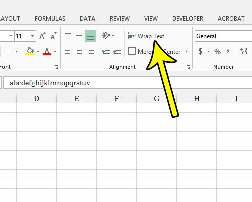
Step 4: Click the Wrap Text button in the Alignment section of the ribbon.
Do you need to print your spreadsheet, but you’re having trouble getting everything to work out properly? This guide will show you some tips that can make a spreadsheet look better when it gets printed on paper. He specializes in writing content about iPhones, Android devices, Microsoft Office, and many other popular applications and devices. Read his full bio here.


