You can use a multi-color fill in Excel 2013 by taking advantage of a gradient fill effect that is found on the Font Settings menu. Our guide below will show you where to find and how to use this fill option so that you can start applying gradient fills to your cells as needed.
How to Do a Gradient Fill in Excel 2013
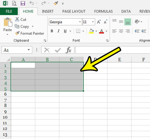
The steps in this guide are going to show you how to fill a cell or selection of cells in Excel 2013 with a gradient. You will be able to select from a few options of gradients that are available in Excel 2013. Step 1: Open your spreadsheet in Excel 2013. Step 2: Select the cell(s) to which you would like to apply the gradient fill.
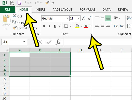
Step 3: Click the Home tab at the top of the window, then click the small Font Settings button at the bottom-right corner of the Font section of the ribbon.
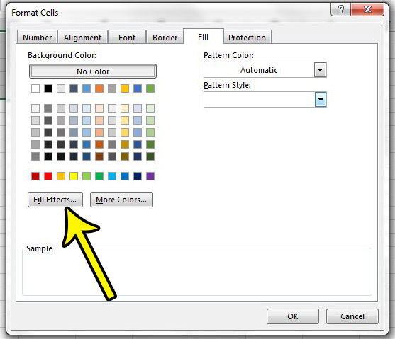
Step 4: Click the Fill tab at the top of the window.
Step 5: Click the Fill Effects button.
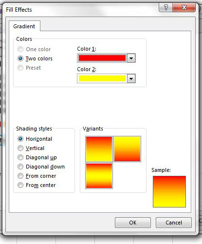
Step 6: Select the colors and shading style for your gradient fill, then click the OK button at the bottom of the window.
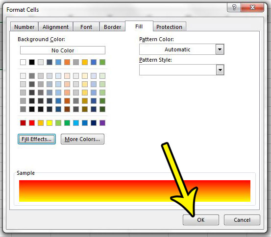
Step 7: Click the OK button to apply your gradient fill to the selected cells.
Are you having difficulty getting your spreadsheet to print the way that you need? Read our Excel printing guide for some tips and tricks that will aid you in printing spreadsheets that fit easily on a page and are simpler to read. He specializes in writing content about iPhones, Android devices, Microsoft Office, and many other popular applications and devices. Read his full bio here.